Interactive Distance Relay Protection Tool - Features & Demonstration

Understanding distance relay protection can be complex, but with the right tools, it becomes an intuitive and interactive process. In this blog post, I explore a newly developed tool that simplifies the analysis of distance relay protection concepts, helping engineers and students grasp the fundamentals and perform real-time calculations.

Watch the video here:

Key Features of the Tool

1. Real-Time Impedance Calculation

The tool starts with the load impedance using voltages and currents under load according to the formula:

$$Z = \frac{V_load}{I_load}$$

Where:

• ${V_load}$ = Voltage (magnitude and angle for each phase under load)
• ${I_load}$ = Current (magnitude and angle for each phase under load)

Users can visualize the impact of changes to these parameters on the impedance plane. For example:

• Dragging the current vector adjusts impedance values instantaneously.
• Manipulating phase voltages reflects on impedance zones immediately, providing a clear picture of relay behavior.

2. Impedance Zones and Relay Reach

The tool provides clear, color-coded visualization of different relay impedance zones (Zone 1, Zone 2, Zone 3). This helps to determine:

• Whether the impedance is within the protection zone.
• Relay behavior for short-circuit and load conditions.

For example:

• Zone 1 is typically configured for instantaneous protection of faults covering 80% of the line.
• Zone 2 and Zone 3 provide time-delayed backup protection for further faults on adjacent sections.

The tool ensures accurate representation of relay characteristics and their alignment with system impedance.

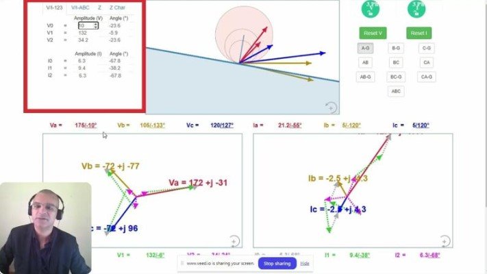
3. Symmetrical Components Analysis

At the bottom panel, the tool displays zero ($I_0$), positive ($I_1$), and negative ($I_2$) sequence currents and voltages, which are essential for analyzing unbalanced faults. The symmetrical components are calculated as:

$$\begin{aligned} & I_0 = \frac{I_a + I_b + I_c}{3} \\ & I_1 = \frac{I_a + a I_b + a^2 I_c}{3} \\ & I_2 = \frac{I_a + a^2 I_b + a I_c}{3} \end{aligned}$$

Where $$a = e^{j120^\circ}$$.

This capability is crucial for understanding fault behavior and deriving relay settings for unbalanced faults.

4. Fault Simulation

Simulating various fault types is one of the most powerful features of this tool. Users can select fault types, including:

• Single-line-to-ground faults (e.g., A-N, B-N, C-N).
• Phase-to-phase faults (e.g., A-B, B-C, C-A).
• Double-line-to-ground faults.
• Three-phase faults.

These fault types affect relay operation and can be studied directly on the impedance plane. For example:

• A-N fault: Creates a shift in the impedance locus to Zone 1 due to a reduction in impedance seen by the relay.

5. Interactive Controls and Visualization

Key interactive features include:

• Adjusting voltage magnitudes and angles for each phase.
• Changing current magnitudes and angles to simulate system conditions.
• Zooming and panning within the impedance plane for detailed inspection.

These features enable users to study specific relay scenarios with precision.

Practical Applications of the Tool

This tool is ideal for:

• Relay Setting Calculations: Adjust relay zones to match system parameters, ensuring accurate operation during faults.
• Fault Analysis: Observe the impact of system faults on relay behavior and impedance zones.
• Educational Use: Visualize concepts like impedance zones, symmetrical components, and fault conditions, making it invaluable for students and engineers in training.

Example: Adjusting Line Parameters

If the protected line impedance is $Z_L = 8 \, \Omega$ at an angle of $80^\circ$, and the line is shortened to half its length, the new impedance becomes $Z_L = 4 \, \Omega$. The tool automatically updates the impedance plane and zone boundaries to reflect this change, ensuring the relay remains correctly set.

Symmetrical Components and K Factor

The tool calculates the K factor, which is used in ground fault detection and is derived as:

$$K = \frac{Z_0 - Z_1}{Z_1}$$

Where:

• $Z_0$ = Zero-sequence impedance
• $Z_1$ = Positive-sequence impedance

By experimenting with $K$, users can observe its impact on relay settings and fault detection capabilities.

Reset and Replay Functionality

The reset buttons allow users to restore voltage and current settings to default values, creating a clean slate for new simulations. This feature is particularly useful for iterative studies and demonstrations.

Conclusion

This interactive tool is a game-changer for distance relay protection studies. It bridges the gap between theoretical understanding and practical application, offering a hands-on approach to mastering impedance, fault analysis, and relay behavior.

Your feedback is invaluable—let me know in the comments if you have any suggestions or ideas for improving this tool!

---

By combining theoretical depth with practical simulation capabilities, this tool is a must-have for relay engineers and students.